Vẽ biểu đồ 2 cột Y trong excell 2007 - secondary axis in a chart

Vẽ biểu đồ 2 cột Y trong excell 2007-

Add or remove a secondary axis in a chart

http://office.microsoft.com/en-001/excel-help/add-or-remove-a-secondary-axis-in-a-chart-HP001234165.aspx

When the values in a 2-D chart vary widely from data series to data series, or when you have mixed types of data (for example, price and volume), you can plot one or more data series on a secondary vertical (value) axis. The scale of the secondary vertical axis reflects the values for the associated data series.

After you add a secondary vertical axis to a 2-D chart, you can also add a secondary horizontal (category) axis, which may be useful in an xy (scatter) chart or bubble chart.

To help distinguish the data that is plotted along the secondary axis, you can change the chart type for just one data series. For example, you could change one data series to a line chart.

 IMPORTANT   To complete the following procedures, you must have an existing 2-D chart. Secondary axes are not supported in 3-D charts. For more information about how to create a chart, see Create a chart.

What do you want to do?

• Add a secondary vertical axis
• Add a secondary horizontal axis
• Change the chart type of a data series
• Remove a secondary axis

Add a secondary vertical axis

You can plot data on a secondary vertical axis one data series at a time. To plot more than one data series on the secondary vertical axis, repeat this procedure for each data series that you want to display on the secondary vertical axis.

1. In a chart, click the data series that you want to plot on a secondary vertical axis, or do the following to select the data series from a list of chart elements:

1. Click the chart.

This displays the Chart Tools, adding the Design, Layout, and Format tabs.

2. On the Format tab, in the Current Selection group, click the arrow in the Chart Elements box, and then click the data series that you want to plot along a secondary vertical axis.

2. On the Format tab, in the Current Selection group, click Format Selection.

The Format Data Series dialog box is displayed.

 NOTE   If a different dialog box is displayed, repeat step 1 and make sure that you select a data series in the chart.

3. On the Series Options tab, under Plot Series On, click Secondary Axis and then click Close.

A secondary vertical axis is displayed in the chart.

4. To change the display of the secondary vertical axis, do the following:

1. On the Layout tab, in the Axes group, click Axes.
2. Click Secondary Vertical Axis, and then click the display option that you want.

5. To change the axis options of the secondary vertical axis, do the following:

1. Right-click the secondary vertical axis, and then click Format Axis.
2. Under Axis Options, select the options that you want to use.

 TIP   To help distinguish the secondary axis, you can change the chart type for just one data series. For example, you can change one data series to a line chart. For more information, see Present your data in a combination chart.

 TOP OF PAGE

Add a secondary horizontal axis

To complete this procedure, you must have a chart that displays a secondary vertical axis. To add a secondary vertical axis, see Add a secondary vertical axis.

1. Click a chart that displays a secondary vertical axis.

This displays the Chart Tools, adding the Design, Layout, and Format tabs.

2. On the Layout tab, in the Axes group, click Axes.

3. Click Secondary Horizontal Axis, and then click the display option that you want.

 TOP OF PAGE

Change the chart type of a data series

1. In a chart, click the data series that you want to change, or do the following to select the data series from a list of chart elements:

1. Click the chart.

This displays the Chart Tools, adding the Design, Layout, and Format tabs.

2. On the Format tab, in the Current Selection group, click the arrow in the Chart Elements box, and then click the data series that you want to change.

2. On the Design tab, in the Type group, click Change Chart Type.

3. Click a chart type in the first box, and then click the chart subtype that you want to use in the second box.

 TOP OF PAGE

Remove a secondary axis

1. Click the chart that displays the secondary axis that you want to remove.

This displays the Chart Tools, adding the Design, Layout, and Format tabs.

2. Do one of the following:

• On the Layout tab, in the Axes group, click Axes, click Secondary Vertical Axis or Secondary Horizontal Axis, and then click None.

• Click the secondary axis that you want to delete, and then press DELETE.

• Right-click the secondary axis, and then click Delete.

 TIP   You can also remove secondary axes immediately after you add them by clicking Undo  on the Quick Access Toolbar, or by pressing CTRL+Z.

__________________________________________________________________________________________________

bài tham khảo 2: Vẽ biểu đồ 2 cột Y trong excell 2007- MS Excel: Create a chart with two Y-axes and one shared X-axis in Excel 2007

Question: How do I create a chart in Excel that has two Y-axes and one shared X-axis in Microsoft Excel 2007?

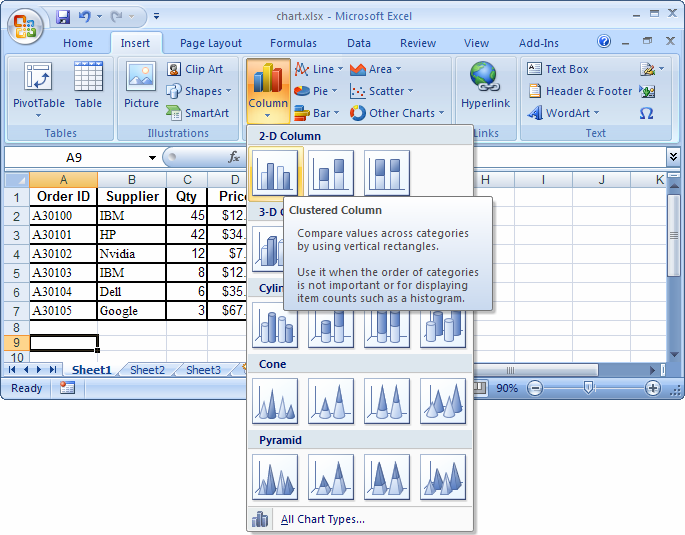
Answer:First, select the Insert tab from the toolbar at the top of the screen. In the Charts group, click on the Column button and select the first chart (Clustered Column) under 2-D Column.

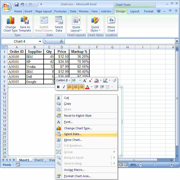
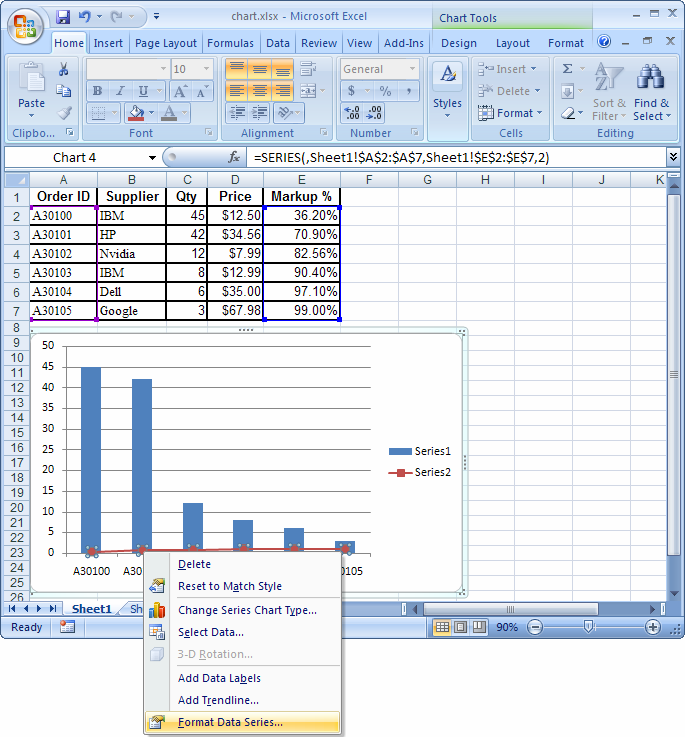
A blank chart object should appear in your spreadsheet. Right-click on this chart object and choose "Select Data..." from the popup menu.

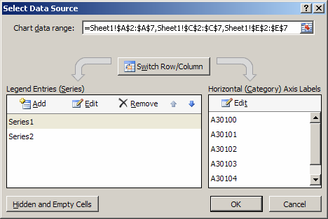
When the Select Data Source window appears, we need to enter the data that we want to graph. In this example, we want column A to represent our X-axis and column C to represent our primary Y-axis (left side) and column E to represent our secondary Y-axis (right side). One more complication to this example is that our data is not all in adjacent cells, so we need to select columns A, C, and E separated by commas.

To do this, highlight cells A2 to A7 then type a comma, then highlight cells C2 to C7, then type another comma, and the highlight cells E2 to E7. You should see the following in your Chart data range box:

=Sheet1!$A$2:$A$7,Sheet1!$C$2:$C$7,Sheet1!$E$2:$E$7

Click on the OK button.

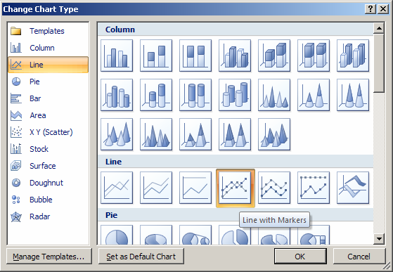
Now, right-click on one of the data points for Series2 and select "Change Series Chart Type" from the popup menu.

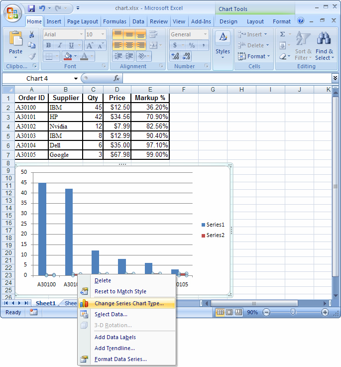
When the Change Chart Type window appears, select the 4th chart under the Line Chart section. Click on the OK button.

Now when you view the chart, you should see that Series 2 has changed to a line graph. However, we still need to set up a secondary Y-axis as Series 2 is currently using the primary Y-axis to display its data.

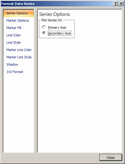
To do this, right-click on one of the data points for Series 2 and select "Format Data Series" from the popup menu.

When the Format Data Series window appears, select the "Secondary Axis" radio button. Click on the Close button.

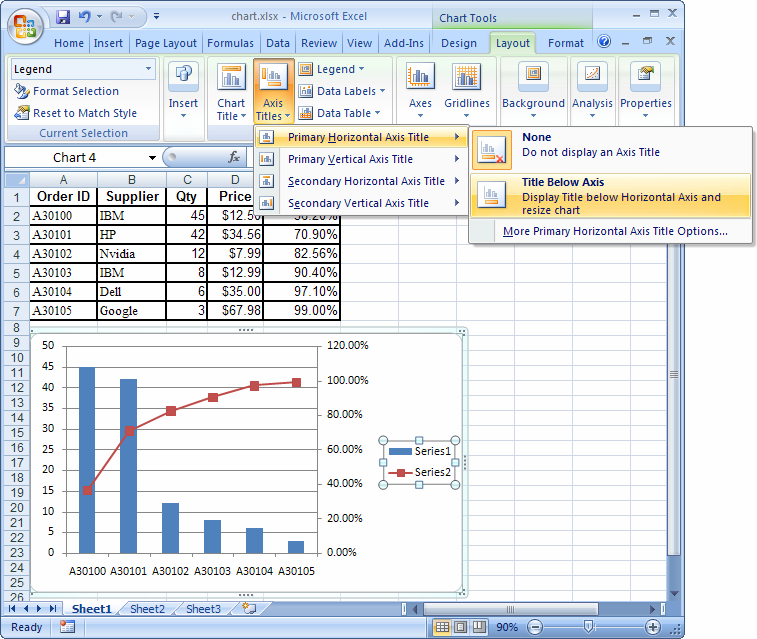
Now, if you want to add axis titles, select the chart and a Layout tab should appear in the toolbar at the top of the screen.

Click on the Layout tab. Then select Axis Titles > Primary Horizontal Axis Title > Title Below Axis.

An Axis Title at the bottom of the graph should appear, just overwrite "Axis Title" with the text that you'd like to see.

Next, under the Layout tab in the toolbar, select Axis Titles > Primary Vertical Axis Title > Horizontal Title.

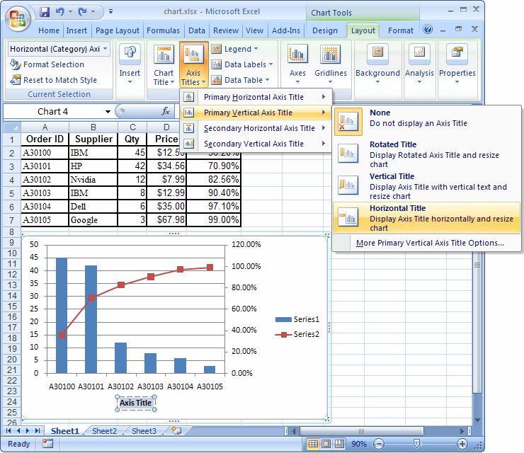
An Axis Title to the left of the graph should appear, just overwrite "Axis Title" with the text that you'd like to see.

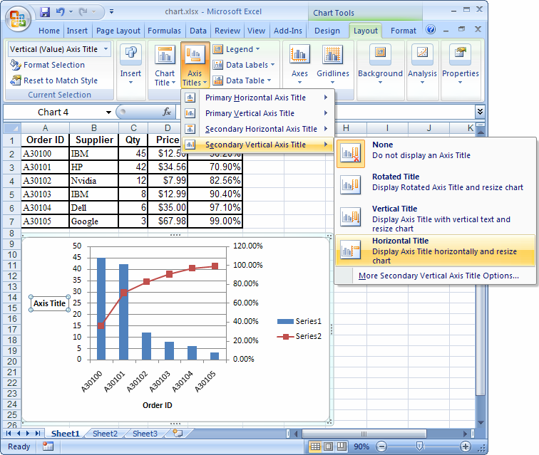
Next, under the Layout tab in the toolbar, select Axis Titles > Secondary Vertical Axis Title > Horizontal Title.

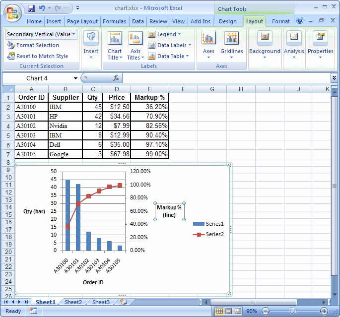
Now, you should see that your chart is designed with a common X-axis and 2 different Y-axes.

http://www.techonthenet.com/excel/charts/2_y_axes.php